Portfolio Balancing with Historical Stock Data

Following last weeks' post (Python for the Finance Industry). This post is to demonstrate a method of determining an optimized portfolio based on historical stock price data.

First of all while attempting to tackle this problem, I stumbled across many very informative articles in which based on what I learned throughout reading them, and trying to replicate their findings with the ASX stocks' data.

• Ricky Kim (Efficient Frontier Portfolio Optimisation in Python)
• Bernard Brenyah (Markowitz’s Efficient Frontier in Python)

Now I will not be going into how Markowit'z Efficient Frontier Portfolio Optimization & Sharpe Ratios works as these techniques are extremely well documented across this internet and very easily found. This post will be for implementing these techniques in Python to apply them to an ASX based portfolio.

Picking up from the end of the previous post, we had just plotted the percentage change over the time period for our stocks' data. For the sake of this post we will be using a technique called random optimization, where will be taking a number of random attempts and selecting the best one. Further posts will show a more detailed approach to this optimization problem.

Now there are multiple steps before we get to the desired outcome of a balanced portfolio.

1. Generate X number of 'random' portfolios,
2. Rate their performance against one another,
3. Pick the desired solution.

To generate random portfolios, we define a function such that we can pass it differing variables as to tweak our outcomes in the future.

 1
 2
 3
 4
 5
 6
 7
 8
 9
10
11
12

def generate_portfolios(num_portfolios,average_returns,covariance_matrix,risk_free_rate):
    results = np.zeros((3,num_portfolios))
    weights_record = []
    for portfolio in range(num_portfolios):
        weights = np.random.random(len(companies) - 1)
        weights /= np.sum(weights)
        weights_record.append(weights)
        returns, volatility = portfolio_performance(weights,average_returns,covariance_matrix)
        results[0,portfolio] = volatility
        results[1,portfolio] = returns
        results[2,portfolio] = (returns - risk_free_rate) / volatility
    return results, weights_record

To step through this function:

1. Define empty location for our portfolio performance results to be stored along with recording weights so we can extract them once selected,
2. For each portfolio to be generated, give a random 'weighting' for each of the company that we have historical data on (eg, 23% NAB.AX),
3. Even out the distribution of the weights such that the sum of the weightings is 100% (eg, total budget),
4. Record the weightings generated in our memory location,
5. Determine the performance of our randomly generated portfolio (more on that soon),
6. Fill in the portfolio performance results for this generated portfolio and repeat for X number of portfolios.

In step 5 above, we have to determine how to rank the generated portfolios against each other to work out how to filter our results. To do this, we calculate volatility of the portfolio using the following formula:

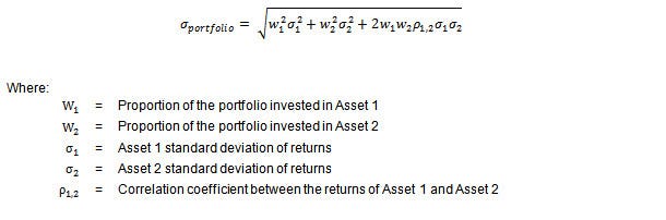
Bernard Brenyah, whom I mentioned at the beginning of the post, has provided a clear explanation of how the above formula can be expressed in matrix calculation in one of his blog posts. In which we just take the matrix calculation and multiply by 253 for number of trading days in Australia.

1
2
3
4
5

def portfolio_performance(weights,average_returns,covariance_matrix):
    returns = np.sum(weights*average_returns) * 253
    variance = np.dot(weights.T,np.dot(covariance_matrix,weights))
    volatility = np.sqrt(variance) * np.sqrt(253)
    return returns, volatility

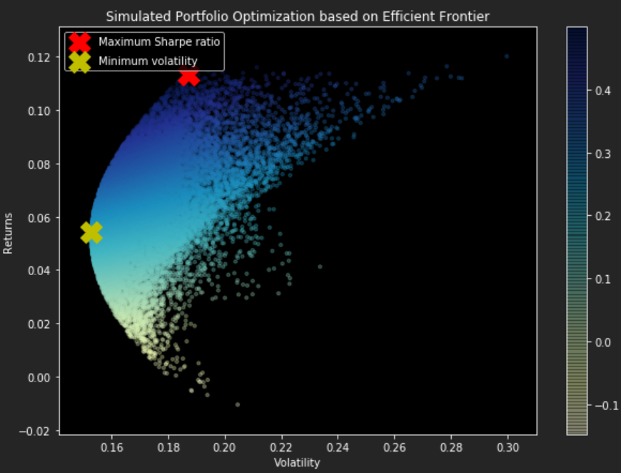
Now that we have X number of randomly generated portfolios, all ranked against one another, it's time to plot so that our results can be visualized.

 1
 2
 3
 4
 5
 6
 7
 8
 9
10
11
12
13
14
15
16
17
18
19
20
21
22
23
24
25
26
27
28
29
30
31
32
33
34
35
36

def display_random_efficient_frontier(average_returns,covariance_matrix,num_portfolios,risk_free_rate):
    results, weights = generate_portfolios(num_portfolios,average_returns,covariance_matrix,risk_free_rate)

    max_sharpe_index = np.argmax(results[2])
    max_volatility = results[0,max_sharpe_index]
    max_return = results[1,max_sharpe_index]
    max_sharpe_allocations = allocations(max_sharpe_index,weights,stocks_df).T

    print("MAX SHARPE RATIO\n")
    print("Return: {0:.2f}".format(max_return))
    print("Volatility: {0:.2f}".format(max_volatility))
    print(max_sharpe_allocations)

    min_vol_index = np.argmin(results[0])
    min_volatility = results[0,min_vol_index]
    min_return = results[1,min_vol_index]
    min_vol_allocations = allocations(min_vol_index,weights,stocks_df).T

    print("\nMINIMUM VOLATILITY\n")
    print("Return: {0:.2f}".format(min_return))
    print("Volatility: {0:.2f}".format(min_volatility))
    print(min_vol_allocations)

    plt.figure(figsize=(10, 7))
    plt.scatter(results[0,:],results[1,:],c=results[2,:],cmap='YlGnBu', marker='o', s=10, alpha=0.3)
    plt.colorbar()
    plt.scatter(max_volatility,max_return,marker='X',color='r',s=400, label='Maximum Sharpe ratio')
    plt.scatter(min_volatility,min_return,marker='X',color='y',s=400, label='Minimum volatility')
    plt.title('Simulated Portfolio Optimization based on Efficient Frontier')
    plt.xlabel('Volatility')
    plt.ylabel('Returns')
    plt.legend(labelspacing=0.8)

def allocations(index,weights,stocks_df):
    allocation = pd.DataFrame(weights[index],index=stocks_df.columns,columns=['allocation'])
    return allocation

Using the above function 'display_random_efficient_frontier', this will determine our max sharpe ratio portfolio generated and the minimum volatility portfolio with their respective returns. Now it is entirely up to the trader on how much risk they are willing to take on board with their portfolio. With the settings below in conjunction with the previously defined functions and stock data to generate the portfolios (risk free rate determined from this website).

1
2
3
4
5
6
7

returns = stocks_df.pct_change()
mean_returns = returns.mean()
cov_matrix = returns.cov()
num_portfolios = 25000
risk_free_rate = 0.01977

display_random_efficient_frontier(mean_returns,cov_matrix,num_portfolios,risk_free_rate)

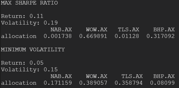
With the two portfolios determined, the one gives us the best risk-adjusted (as long as the trader is prepared to take the risk) is the one with the maximum Sharpe ratio, allocating a 67% portion to WOW and 32% to BHP, as these stocks were quite volatile from the daily percentage change calculations.

On the other hand, the minimum volatility portfolio is reflecting the more stable of the stocks from the daily percentage change calculations distributing portions over NAB and TLS due to their stability from the percentage change calculations and reducing the portion to WOW.