3D Gradient Descent in Python
Posted on Wed 26 February 2020 in Python • 40 min read
Visualising gradient descent in 3 dimensions
Building upon our terrain generator from the blog post: https://jackmckew.dev/3d-terrain-in-python.html, today we will implement a demonstration of how gradient descent behaves in 3 dimensions and produce an interactive visualisation similar to the terrain visualisation. Note that my understanding of gradient descent this does not behave in the similar manner as the gradient descent function used heavily in optimisation problems, although this does make for a demonstration.
What is Gradient Descent
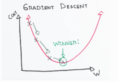
The premise behind gradient descent is at a point in an a 'function' or array, you can determine the minimum value or maximum value by taking the steepest slope around the point till you get to the minimum/maximum. As optimising functions is one of the main premises behind machine learning, gradient descent is used to reduce computation time & resources.Image Source
What can I use this for?
At it's core, gradient descent is a optimisation algorithm used to minimise a function. The benefit of gradient shines when searching every single possible combination isn't feasible, so taking an iterative approach to finding the minimum is favourable.
In machine learning, we use gradient descent to update the parameters of our model. Parameters refer weights on training data, coefficients in Linear Regression, weights in neural networks and more.
How?
A way of imagining this is if you are at the top of a hill, and want to get to the bottom in the quickest way possible, if you take a step in each time in the direction of the steepest slope, you should hopefully get to the bottom a quick as possible.
What could go wrong?
The common pitfalls behind gradient descent is that the algorithm can get 'stuck' within holes, ridges or plateaus meaning the algorithm converges on a local minimum, rather than the global minimum. Another problem being the step size can be difficult to estimate before calculation, in that if you take too small of steps it will take too long to converge.
Let's get started!
First of all, we need to import all the packages we will need to use, then we will use the numpy array from last time which we generated with Perlin Noise. Next we will find the global maximum and minimum, and plot this all on a 2D contour plot. The maximum (highest point) is show by the red dot, while the minimum (lowest point) is shown by the yellow dot.
from IPython.core.display import HTML
import plotly
import plotly.graph_objects as go
import noise
import numpy as np
import matplotlib
from mpl_toolkits.mplot3d import axes3d
%matplotlib inline
z = world
matplotlib.pyplot.imshow(z,origin='lower',cmap='terrain')

# Find maximum value index in numpy array
indices = np.where(z == z.max())
max_z_x_location, max_z_y_location = (indices[1][0],indices[0][0])
matplotlib.pyplot.plot(max_z_x_location,max_z_y_location,'ro',markersize=15)

# Find minimum value index in numpy array
indices = np.where(z == z.min())
min_z_x_location, min_z_y_location = (indices[1][0],indices[0][0])
matplotlib.pyplot.plot(min_z_x_location,min_z_y_location,'yo',markersize=15)

For our implementation in this blog post, rather than computing the gradient at each point (typical implementation), we will evaluate our array by searching through the 'neighbouring' values around a certain index. Luckily, an answer from pv on Stackoverflow had already solved this problem for us.
# Source: https://stackoverflow.com/questions/10996769/pixel-neighbors-in-2d-array-image-using-python
# This code by pv (https://stackoverflow.com/users/108184/pv), is to find all the adjacent values around a specific index
import numpy as np
from numpy.lib.stride_tricks import as_strided

def sliding_window(arr, window_size):
    """ Construct a sliding window view of the array"""
    arr = np.asarray(arr)
    window_size = int(window_size)
    if arr.ndim != 2:
        raise ValueError("need 2-D input")
    if not (window_size > 0):
        raise ValueError("need a positive window size")
    shape = (arr.shape[0] - window_size + 1,
             arr.shape[1] - window_size + 1,
             window_size, window_size)
    if shape[0] <= 0:
        shape = (1, shape[1], arr.shape[0], shape[3])
    if shape[1] <= 0:
        shape = (shape[0], 1, shape[2], arr.shape[1])
    strides = (arr.shape[1]*arr.itemsize, arr.itemsize,
               arr.shape[1]*arr.itemsize, arr.itemsize)
    return as_strided(arr, shape=shape, strides=strides)

def cell_neighbours(arr, i, j, d):
    """Return d-th neighbors of cell (i, j)"""
    w = sliding_window(arr, 2*d+1)

    ix = np.clip(i - d, 0, w.shape[0]-1)
    jx = np.clip(j - d, 0, w.shape[1]-1)

    i0 = max(0, i - d - ix)
    j0 = max(0, j - d - jx)
    i1 = w.shape[2] - max(0, d - i + ix)
    j1 = w.shape[3] - max(0, d - j + jx)

    return w[ix, jx][i0:i1,j0:j1].ravel()
Now we will implement our function which will calculate the gradient descent of an array from a point in the array with nominated maximum number of steps & size of step.
This works by:
- extracting a smaller subset array of all the values around a specified point (in this post we will start a the maximum point),
- locating the minimum in this array (inferring the greatest slope from the current point),
- move our current location to the minimum
- repeat till the point stays the same as previous step
We also store of all our previous steps in gradient descent in a list such that we can use this to plot later on.
from dataclasses import dataclass

@dataclass
class descent_step:
    """Class for storing each step taken in gradient descent"""
    value: float
    x_index: float
    y_index: float

def gradient_descent_3d(array,x_start,y_start,steps=50,step_size=1,plot=False):
    # Initial point to start gradient descent at
    step = descent_step(array[y_start][x_start],x_start,y_start)

    # Store each step taken in gradient descent in a list
    step_history = []
    step_history.append(step)

    # Plot 2D representation of array with startng point as a red marker
    if plot:
        matplotlib.pyplot.imshow(array,origin='lower',cmap='terrain')
        matplotlib.pyplot.plot(x_start,y_start,'ro')
    current_x = x_start
    current_y = y_start

    # Loop through specified number of steps of gradient descent to take
    for i in range(steps):
        prev_x = current_x
        prev_y = current_y

        # Extract array of neighbouring cells around current step location with size nominated
        neighbours=cell_neighbours(array,current_y,current_x,step_size)

        # Locate minimum in array (steepest slope from current point)
        next_step = neighbours.min()
        indices = np.where(array == next_step)

        # Update current point to now be the next point after stepping
        current_x, current_y = (indices[1][0],indices[0][0])
        step = descent_step(array[current_y][current_x],current_x,current_y)

        step_history.append(step)

        # Plot each step taken as a black line to the current point nominated by a red marker
        if plot:
            matplotlib.pyplot.plot([prev_x,current_x],[prev_y,current_y],'k-')
            matplotlib.pyplot.plot(current_x,current_y,'ro')

        # If step is to the same location as previously, this infers convergence and end loop
        if prev_y == current_y and prev_x == current_x:
            print(f"Converged in {i} steps")
            break
    return next_step,step_history
Next, to ensure that we get to our global minimum in the end, we loop through each step size until we reach a step size large enough to reach the global minimum.
Note that this is possibly not feasible in some implementations of gradient descent, but for demonstration purposes we will use it here
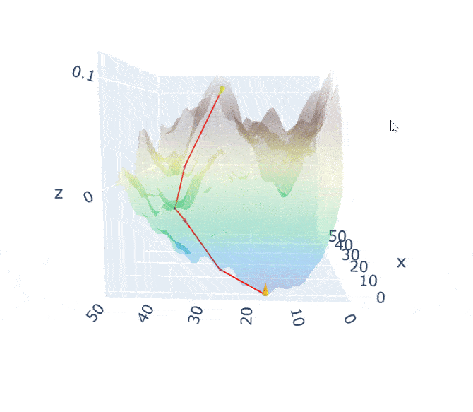
We then randomise a point for the algorithm to start at and then compute the gradient descent until we have a large enough step size to reach the global minimum (see below for a step size smaller than the required size).
np.random.seed(42)
global_minimum = z.min()
indices = np.where(z == global_minimum)
print(f"Target: {global_minimum} @ {indices}")

step_size = 0
found_minimum = 99999

# Random starting point
start_x = np.random.randint(0,50)
start_y = np.random.randint(0,50)

# Increase step size until convergence on global minimum
while found_minimum != global_minimum:
    step_size += 1
    found_minimum,steps = gradient_descent_3d(z,start_x,start_y,step_size=step_size,plot=False)

print(f"Optimal step size {step_size}")
found_minimum,steps = gradient_descent_3d(z,start_x,start_y,step_size=step_size,plot=True)
print(f"Steps: {steps}")

Moving from each point to the next is typically represented as a vector, in our case, this will be in 3D space. In 2D space, you would use a quiver plot to show this, in 3D, you can use a Cone Plot. To calculate the vector between each of our steps, we again turn to Stackoverflow from an answer by teclnol.
# Source https://stackoverflow.com/questions/51272288/how-to-calculate-the-vector-from-two-points-in-3d-with-python

def multiDimenDist(point1,point2):
   #find the difference between the two points, its really the same as below
   deltaVals = [point2[dimension]-point1[dimension] for dimension in range(len(point1))]
   runningSquared = 0
   #because the pythagarom theorm works for any dimension we can just use that
   for coOrd in deltaVals:
       runningSquared += coOrd**2
   return runningSquared**(1/2)
def findVec(point1,point2,unitSphere = False):
  #setting unitSphere to True will make the vector scaled down to a sphere with a radius one, instead of it's orginal length
  finalVector = [0 for coOrd in point1]
  for dimension, coOrd in enumerate(point1):
      #finding total differnce for that co-ordinate(x,y,z...)
      deltaCoOrd = point2[dimension]-coOrd
      #adding total difference
      finalVector[dimension] = deltaCoOrd
  if unitSphere:
      totalDist = multiDimenDist(point1,point2)
      unitVector =[]
      for dimen in finalVector:
          unitVector.append( dimen/totalDist)
      return unitVector
  else:
      return finalVector
Finally, we build a function that can generate 3D plots with Plotly, similar to the terrain visualisation with the steps in gradient descent visualised as cones and lines.
def generate_3d_plot(step_history):
    # Initialise empty lists for markers
    step_markers_x = []
    step_markers_y = []
    step_markers_z = []
    step_markers_u = []
    step_markers_v = []
    step_markers_w = []

    for index, step in enumerate(step_history):
        step_markers_x.append(step.x_index)
        step_markers_y.append(step.y_index)
        step_markers_z.append(step.value)

        # If we haven't reached the final step, calculate the vector between the current step and the next step
        if index < len(steps)-1:
            vec1 = [step.x_index,step.y_index,step.value]
            vec2 = [steps[index+1].x_index,steps[index+1].y_index,steps[index+1].value]

            result_vector = findVec(vec1,vec2)
            step_markers_u.append(result_vector[0])
            step_markers_v.append(result_vector[1])
            step_markers_w.append(result_vector[2])
        else:
            step_markers_u.append(0.1)
            step_markers_v.append(0.1)
            step_markers_w.append(0.1)

    # Include cones at each marker to show direction of step, scatter3d is to show the red line between points and surface for the terrain
    fig = go.Figure(data=[
        go.Cone(
        x=step_markers_x,
        y=step_markers_y,
        z=step_markers_z,
        u=step_markers_u,
        v=step_markers_v,
        w=step_markers_w,
        sizemode="absolute",
        sizeref=2,
        anchor='tail'),

        go.Scatter3d(
        x=step_markers_x,
        y=step_markers_y,
        z=step_markers_z,
        mode='lines',
        line=dict(
            color='red',
            width=2
        )),

        go.Surface(colorscale=terrain,z=world,opacity=0.5)])


    # Z axis is limited to the extent of the terrain array
    fig.update_layout(
        title='Gradient Descent Steps',
        scene = dict(zaxis = dict(range=[world.min(),world.max()],),),)
    return fig

# Generate 3D plot from previous random starting location
fig = generate_3d_plot(steps)
HTML(plotly.offline.plot(fig, filename='random_starting_point_3d_gradient_descent.html',include_plotlyjs='cdn'))
To demonstrate how gradient descent can be stuck, by setting the gradient descent algorithm to start a the maximum point with a step size of 5, we can see how it falls straight into the nearest ditch (local minima) but then cannot get out of it.
found_minimum,steps = gradient_descent_3d(z,max_z_x_location,max_z_y_location,step_size=5,plot=True)
fig = generate_3d_plot(steps)
HTML(plotly.offline.plot(fig, filename='maximum_starting_point_step_size_5_3d_gradient_descent.html',include_plotlyjs='cdn'))
