Australia Post Codes Connected
Posted on Mon 29 May 2023 in Python • 4 min read
Have you ever wondered what the sequence to postcodes is? Ever wondered who your postcode neighbour was? I definitely have, so I've built a visualisation to do exactly that, and made it interactive for everybody to play around with!
Before we get into any of the processing, let's take a look at the interactive map!
For those on mobile, ensure to press the full screen button underneath the layers button!
# This is to display the map at the beginning of the blog post
m
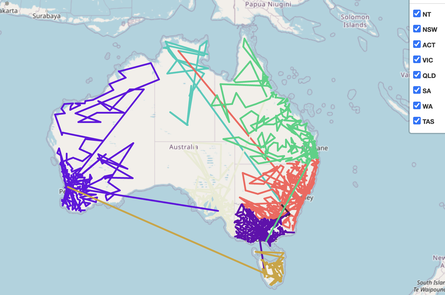
For those that aren't able to see the interactive version, here's a photo :)
First of all, we'll need to get the data of each postcode in Australia and a relevant latitude/longitude such that we can process and plot it. A big thank you to Matthew Proctor who has already gone through this data gathering for us!
Now let's look into what data points have come along in this dataset.
import geopandas as gpd
df = gpd.pd.read_csv('../data/australian_postcodes.csv')
df.iloc[:5,:6]
Looks like there's a lot of data points with each postcode, so before we begin any further cleaning of the data, let's plot it to see the geographic extent of how far this data goes.
gdf = gpd.GeoDataFrame(
    df, geometry=gpd.points_from_xy(df.long, df.lat), crs="EPSG:4326"
)
gdf.plot()

Woah, looks like it's even got coordinates in there for all the territories of Australia (there's 10 of them!), it also seems from looking at the data above, there's lots of duplicates in locations & postcodes, so let's clean these up.
We do this through the process of:
- Remove any duplicate postcodes (we keep the first)
- Remove any duplicate geometries (keeping the first again)
This should ensure that we have unique postcodes, with unique geometries.
# There's duplicate postcodes, and geometries that need to be removed
gdf = gdf.drop_duplicates(subset=['postcode']).drop_duplicates(subset='geometry')
Next up, since we aren't overly concerned about the territories of Australia, and more interested in the mainland postcodes, let's filter our points such that they exist in a bounding box of Australia.
# http://bboxfinder.com/#-45.559737,109.346924,-10.454727,157.862549

def filter_gdf_by_bounding_box(gdf,minimum_longitude,minimum_latitude,maximum_longitude,maximum_latitude):
    return gdf.cx[minimum_longitude:maximum_longitude, minimum_latitude:maximum_latitude]

filtered_gdf = filter_gdf_by_bounding_box(gdf,109.346924,-45.559737,157.862549,-10.454727)

filtered_gdf.plot()

Next up is the part everyone has been waiting for! We want to do a few things here before creating the output dataset:
- We want to draw a line between each postcode
- For each line we want to embed:
- starting postcode & name
- ending postcode & name
- state postcode exists in
from shapely.geometry import LineString

def check_geometry_valid(geometry):
    if geometry.x == 0 or geometry.y == 0:
        return False
    return True

def convert_gdf_to_linestring(gdf):
    gdf = gdf.reset_index()
    linestring_gdf = gpd.GeoDataFrame()

    for index, row in gdf.iterrows():
        current_row = row
        # Skip the first row
        if index > 0:
            previous_row = gdf.iloc[index - 1, :]

            # Ensure geometry valid
            if check_geometry_valid(current_row.geometry) and check_geometry_valid(
                previous_row.geometry
            ):
                # Create a linestring connecting each postcode to one another
                linestring = LineString([previous_row.geometry, current_row.geometry])
                new_line = gpd.GeoDataFrame(
                    [
                        [
                            f"{previous_row['postcode']}-{current_row['postcode']}",
                            f"{previous_row['locality']}-{current_row['locality']}",
                            current_row["state"],
                        ]
                    ],
                    geometry=[linestring],
                    columns=["Postcodes","Localities", "State"],
                    crs="EPSG:4326",
                )
                # Build resulting dataframe line by line
                linestring_gdf = gpd.pd.concat([linestring_gdf, new_line])

    return linestring_gdf


convert_gdf_to_linestring(gdf).head()
Now we should be able to plot this and see how the states connect!
convert_gdf_to_linestring(filtered_gdf).plot('State')

Finally, let's use folium to make this interactive.
import folium
from folium import plugins
import random

# Create an interactive Map instance
m = folium.Map(location=[-27, 135], zoom_start=4, control_scale=True)

# Convert the LineString to GeoJSON
converted_gdf = convert_gdf_to_linestring(filtered_gdf)

# Generate random colours for each state to colour them
states = converted_gdf["State"].unique()
state_colours = {type_val: f"#{random.randint(0, 0xFFFFFF):06x}" for type_val in states}


def style_function(feature):
    state = feature["properties"]["State"]
    color = state_colours.get(state, "blue")
    return {"color": color, "fillColor": color}


# Add the LineString to the map as a GeoJSON layer
for state in states:
    folium.GeoJson(
        converted_gdf[converted_gdf["State"] == state].to_json(),
        name=state,
        style_function=style_function,
        tooltip=folium.GeoJsonTooltip(fields=["Postcodes", "Localities", "State"]),
    ).add_to(m)

# Add a layer control to toggle the visibility of the LineString layer
folium.LayerControl().add_to(m)
plugins.Fullscreen(
    position="topright",
    title="FULL SCREEN ON",
    title_cancel="FULL SCREEN OFF",
    force_separate_button=True,
).add_to(m)