Following last 2 weeks’ posts (Python for the Finance Industry & Portfolio Balancing with Historical Stock Data), we now know how to extract historical records on stock information from the ASX through an API, present it in a graph using matplotlib, and how to balance a portfolio using randomly generated portfolios.
This post is to demonstrate a method in balancing portfolios that does not depend on generating random portfolios, but rather mathematically determining the extremities of boundaries for effective portfolios using the SciPy optimize function (similar to that of Excel's 'solver').
Returning to last weeks' post when the budget allocations to assets were determined from randomly generated portfolios, it was presented on the graph below:
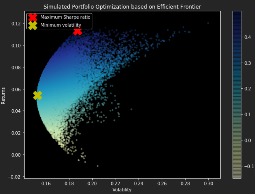
From this plot, it can be visualized that it forms an arch line between the yellow and red crosses. This line is called the efficient frontier. The efficient frontier represents the set of optimal portfolios that offer the highest expected return for a defined level of risk or the lowest risk for a given level of expected return. Simply this means, all the dots (portfolios) to the right of the line will give you a higher risk for the same returns.
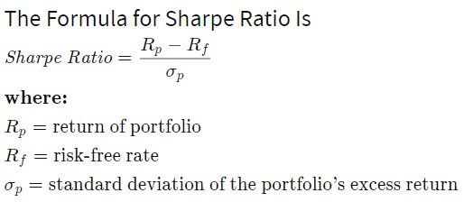
First of all we must mathematically determine the portfolio with the maximum Sharpe ratio as the greater a portfolio's Sharpe ratio, the better it's risk-adjusted performance. Sharpe ratio is calculated using the formula below:
To find the maximum of the Sharpe Ratio programmatically we follow these steps:
- Firstly, define the formula as the function neg_sharpe_ratio (take note that to find the maximum of function in SciPy, we use the minimize function with an inverse sign),
- In the max_sharpe_ratio function, define arguments to be passed into the SciPy minimize function:
- neg_sharpe_ratio: function to be minimized,
- num*[1/num_assets]: initial guess which is evenly distributed array of values,
- Arguments that are to be passed into the objective function (neg_sharpe_ratio),
- Method of Sequential Lease Squares Programming, there are many others which can be seen here,
- Bounds: between 0% and 100% of our budget allocation,
- Constraints: given as a dictionary, 'eq' type for equality and 'fun' for the anonymous function which limits the total summed asset allocation to 100% of the budget.
- The result from the minimize function is returned as a OptimizeResult type.
 1
 2
 3
 4
 5
 6
 7
 8
 9
10
11
12 | def neg_sharpe_ratio(weights, average_returns, covariance_matrix, risk_free_rate):
returns, volatility = portfolio_performance(weights, average_returns, covariance_matrix)
return -(returns - risk_free_rate) / volatility
def max_sharpe_ratio(average_returns, covariance_matrix,risk_free_rate):
num_assets = len(average_returns)
args = (average_returns, covariance_matrix, risk_free_rate)
constraints = ({'type': 'eq', 'fun': lambda x: np.sum(x) - 1})
bound = (0,1)
bounds = tuple(bound for asset in range(num_assets))
result = sco.minimize(neg_sharpe_ratio,num_assets*[1/num_assets,],args=args,method='SLSQP',bounds=bounds,constraints=constraints)
return result
|
Similarly to the maximum sharpe ratio we do the same for determining the minimum volatility portfolio programmatically. We minimise volatility by trying different weightings on our asset allocations to find the minima.
 1
 2
 3
 4
 5
 6
 7
 8
 9
10
11
12
13 | def portfolio_volatility(weights, average_returns, covariance_matrix):
return portfolio_performance(weights, average_returns, covariance_matrix)[1]
def min_variance(average_returns, covariance_matrix):
num_assets = len(average_returns)
args = (average_returns, covariance_matrix)
constraints = ({'type': 'eq', 'fun': lambda x: np.sum(x) - 1})
bound = (0.0,1.0)
bounds = tuple(bound for asset in range(num_assets))
result = sco.minimize(portfolio_volatility, num_assets*[1./num_assets,], args=args, method='SLSQP', bounds=bounds, constraints=constraints)
return result
|
As above, we can also draw a line which depicts the efficient frontier for the portfolios for a given risk rate. Below some functions are defined for computing the efficient frontier. The first function, efficient_return is calculating the most efficient portfolio for a given target return, and the second function efficient frontier is compiling the most efficient portfolio for a range of targets.
 1
 2
 3
 4
 5
 6
 7
 8
 9
10
11
12
13
14
15
16
17
18
19 | def efficient_return(average_returns, covariance_matrix, target):
num_assets = len(average_returns)
args = (average_returns, covariance_matrix)
def portfolio_return(weights):
return portfolio_performance(weights, average_returns, covariance_matrix)[0]
constraints = ({'type': 'eq', 'fun': lambda x: portfolio_return(x) - target},
{'type': 'eq', 'fun': lambda x: np.sum(x) - 1})
bounds = tuple((0,1) for asset in range(num_assets))
result = sco.minimize(portfolio_volatility, num_assets*[1./num_assets,], args=args, method='SLSQP', bounds=bounds, constraints=constraints)
return result
def efficient_frontier(average_returns, covariance_matrix, returns_range):
efficients = []
for ret in returns_range:
efficients.append(efficient_return(average_returns, covariance_matrix, ret))
return efficients
|
Now it's time to plot the efficient frontier on the graph with the randomly selected portfolios to check if they have been calculated correctly. It is also an opportune time to check if the maximum Sharpe ratio and minimum volatility portfolios have been calculated correctly by comparing them to the previously randomly determined portfolios.
 1
 2
 3
 4
 5
 6
 7
 8
 9
10
11
12
13
14
15
16
17
18
19
20
21
22
23
24
25
26
27
28
29
30
31
32
33
34
35
36
37
38
39
40
41
42
43
44
45
46
47
48
49
50
51
52
53
54 | def display_efficient_frontier(average_returns,covariance_matrix,num_portfolios,risk_free_rate):
results, weights = generate_portfolios(num_portfolios,average_returns,covariance_matrix,risk_free_rate)
max_sharpe = max_sharpe_ratio(average_returns,covariance_matrix,risk_free_rate)
max_sharpe_return, max_sharpe_volatility = portfolio_performance(max_sharpe['x'],average_returns,covariance_matrix)
max_sharpe_allocations = allocations_ef(max_sharpe.x,stocks_df).T
print("MAX SHARPE RATIO\n")
print("Return: {0:.2f}".format(max_sharpe_return))
print("Volatility: {0:.2f}".format(max_sharpe_volatility))
print(max_sharpe_allocations)
min_vol = min_variance(average_returns,covariance_matrix)
min_vol_return, min_vol_volatility = portfolio_performance(min_vol['x'],average_returns,covariance_matrix)
min_vol_allocations = allocations_ef(min_vol.x,stocks_df).T
print("\nMINIMUM VOLATILITY\n")
print("Return: {0:.2f}".format(min_vol_return))
print("Volatility: {0:.2f}".format(min_vol_volatility))
print(min_vol_allocations)
an_vol = np.std(returns) * np.sqrt(253)
an_rt = average_returns * 253
for i, txt in enumerate(stocks_df.columns):
print(txt,":","Annuaised return",round(an_rt[i],2),", Annualised volatility:",round(an_vol[i],2))
plt.figure(figsize=(10, 7))
plt.scatter(results[0,:],results[1,:],c=results[2,:],cmap='YlGnBu', marker='o', s=10, alpha=0.3)
plt.colorbar()
plt.scatter(max_sharpe_volatility,max_sharpe_return,marker='X',color='r',s=400, label='Maximum Sharpe ratio')
plt.scatter(min_vol_volatility,min_vol_return,marker='X',color='y',s=400, label='Minimum volatility')
target = np.linspace(min_vol_return, max(an_rt), 50)
efficient_portfolios = efficient_frontier(average_returns, covariance_matrix, target)
plt.plot([p['fun'] for p in efficient_portfolios], target, linestyle='-.', color='white', label='efficient frontier')
plt.title('Calculated Portfolio Optimization based on Efficient Frontier')
plt.xlabel('Volatility')
plt.ylabel('Returns')
plt.legend(labelspacing=0.8)
def allocations_ef(solution,stocks_df):
allocation = pd.DataFrame(solution,index=stocks_df.columns,columns=['allocation'])
return allocation
returns = stocks_df.pct_change()
average_returns = returns.mean()
covariance_matrix = returns.cov()
num_portfolios = 25000
risk_free_rate = 0.01977
display_efficient_frontier(average_returns,covariance_matrix,num_portfolios,risk_free_rate)
|
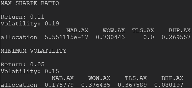
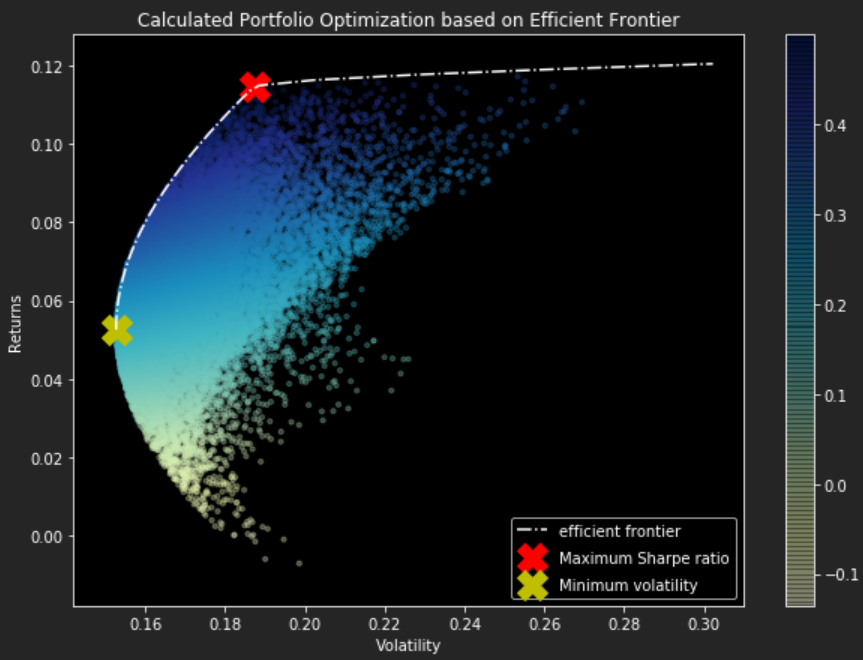
The surprising part is that the calculated result is very close to what we have previously simulated by picking from randomly generated portfolios. The slight differences in allocations between the simulated vs calculated are in most cases less than 1%, which shows how powerful randomly estimating calculations can be albeit sometimes not reliable in small sample spaces.
Rather than plotting every randomly generated portfolio, we can plot the individual stocks on the plot with the corresponding values of each stock's return and risk. This way we can compare how diversification is lowering the risk by optimizing the allocations.
 1
 2
 3
 4
 5
 6
 7
 8
 9
10
11
12
13
14
15
16
17
18
19
20
21
22
23
24
25
26
27
28
29
30
31
32
33
34
35
36
37
38
39
40
41
42
43
44
45
46
47 | def display_efficient_frontier_selected(average_returns,covariance_matrix,risk_free_rate):
max_sharpe = max_sharpe_ratio(average_returns,covariance_matrix,risk_free_rate)
max_sharpe_return, max_sharpe_volatility = portfolio_performance(max_sharpe['x'],average_returns,covariance_matrix)
max_sharpe_allocations = allocations_ef(max_sharpe.x,stocks_df).T
print("MAX SHARPE RATIO\n")
print("Return: {0:.2f}".format(max_sharpe_return))
print("Volatility: {0:.2f}".format(max_sharpe_volatility))
print(max_sharpe_allocations)
min_vol = min_variance(average_returns,covariance_matrix)
min_vol_return, min_vol_volatility = portfolio_performance(min_vol['x'],average_returns,covariance_matrix)
min_vol_allocations = allocations_ef(min_vol.x,stocks_df).T
print("\nMINIMUM VOLATILITY\n")
print("Return: {0:.2f}".format(min_vol_return))
print("Volatility: {0:.2f}".format(min_vol_volatility))
print(min_vol_allocations)
an_vol = np.std(returns) * np.sqrt(253)
an_rt = average_returns * 253
for i, txt in enumerate(stocks_df.columns):
print(txt,":","Annuaised return",round(an_rt[i],2),", Annualised volatility:",round(an_vol[i],2))
plt.figure(figsize=(10, 7))
plt.scatter(an_vol,an_rt,marker='o',s=200)
for i, txt in enumerate(stocks_df.columns):
plt.annotate(txt, (an_vol[i],an_rt[i]), xytext=(10,0), textcoords='offset points')
plt.scatter(max_sharpe_volatility,max_sharpe_return,marker='X',color='r',s=400, label='Maximum Sharpe ratio')
plt.scatter(min_vol_volatility,min_vol_return,marker='X',color='y',s=400, label='Minimum volatility')
target = np.linspace(min_vol_return, max(an_rt), 50)
efficient_portfolios = efficient_frontier(average_returns, covariance_matrix, target)
plt.plot([p['fun'] for p in efficient_portfolios], target, linestyle='-.', color='white', label='efficient frontier')
plt.title('Calculated Portfolio Optimization based on Efficient Frontier')
plt.xlabel('Volatility')
plt.ylabel('Returns')
plt.legend(labelspacing=0.8)
display_efficient_frontier_selected(average_returns,covariance_matrix,risk_free_rate)
|
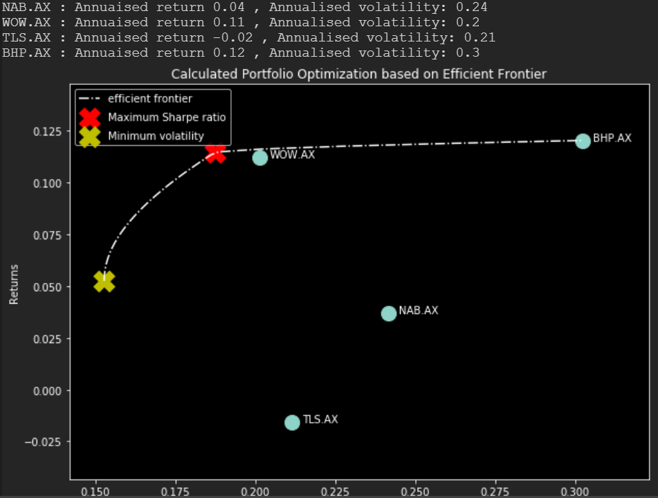
From the plot above, the stock with the highest risk is BHP, which accompanies the highest returns. This shows that if the investor is willing to take the risk than they will be rewarded with the higher return.
This concludes the 3 part series on Python in the finance industry, if there is any topics in particular you would like to see how software can integrate and improve a service/product please feel free to get in touch!