Sentiment Analysis & Text Cleaning in Python with Vader
Posted on Fri 17 July 2020 in Data Science • 8 min read
Sentiment Analysis in Python with Vader
Sentiment analysis is the interpretation and classification of emotions (positive, negative and neutral) within text data using text analysis techniques. Essentially just trying to judge the amount of emotion from the written words & determine what type of emotion. This post we'll go into how to do this with Python and specifically the package Vader https://github.com/cjhutto/vaderSentiment. This post comes from a recent research project I helped out with the University of San Diego for investigating the sentiment of Twitter users in Italy during the pandemic against when the policy changes were enacted (eg, Lockdowns, etc). Sentiment analysis was the step after translating the data, which was detailed on a previous post: https://jackmckew.dev/translating-text-in-python.html.
Find the full source code for the research project at: https://github.com/HDMA-SDSU/Translate-Tweets
As always, first we set up the virtual environment, install any necessary packages and import them. In this post we'll make use of:
- nltk
- pandas
- vader
- wordcloud
We also prepare a few datasets to use later on, stopwords & wordnet. Stop words are words which in English add no meaning to the rest of the setence, for example, the words like the, he, have etc. All these stopwords can be ignored without ruining the meaning of the sentence; although when using pre-computed sentiment analysis libraries removing these words may be of detriment to the determined scores.
Wordnet is used later on for lemmatization (aka stemming), which is the process of bringing words down to their 'root' word. For example, the words car, cars, car's, cars' all share the common 'root' word, car. Note that this can also be of detriment when using pre-computer sentiment analysis libraries.
import pandas as pd
import nltk
import typing
import matplotlib.pyplot as plt
nltk.download('stopwords')
nltk.download('wordnet')
Next up we need a dataset that we can run the sentimment analysis on, for this we use a dataset offered by a stanford course (https://nlp.stanford.edu/sentiment/code.html) which contains ~10,000 rotten tomato reviews (a movie review website). Let's try and find the top positive & negative reviews in this dataset with vader.
# Read in data here
# https://nlp.stanford.edu/sentiment/code.html
text_data = pd.read_table('original_rt_snippets.txt',header=None)
display(text_data.sample(5))
Now that we've downloaded the stopword dataset previously, let's take a look at whats inside it.
# Import english stop words

from nltk.corpus import stopwords
stopcorpus: typing.List = stopwords.words('english')
print(stopcorpus)
Finally it's time to analyse the sentiment with Vader, we need to import the SentimentIntensityAnalzer object to gain access to the polarity score methods inside.
from vaderSentiment.vaderSentiment import SentimentIntensityAnalyzer
sid_analyzer = SentimentIntensityAnalyzer()
To make it easier to interface, let's define some functions which will make it easier to grab all the sentiment values for a specific column in a dataframe. get_sentiment wraps around the analysers polarity scoring method and returns the sentiment score for the specified label. The Vader sentiment analyser method returns a dictionary with the scores for positive, negative, neutral and compound. Next we define the function get_sentiment_scores, which will call get_sentiment function on every value in a certain column and add these values back to the dataframe as a column.
def get_sentiment(text:str, analyser,desired_type:str='pos'):
    # Get sentiment from text
    sentiment_score = analyser.polarity_scores(text)
    return sentiment_score[desired_type]

# Get Sentiment scores
def get_sentiment_scores(df,data_column):
    df[f'{data_column} Positive Sentiment Score'] = df[data_column].astype(str).apply(lambda x: get_sentiment(x,sid_analyzer,'pos'))
    df[f'{data_column} Negative Sentiment Score'] = df[data_column].astype(str).apply(lambda x: get_sentiment(x,sid_analyzer,'neg'))
    df[f'{data_column} Neutral Sentiment Score'] = df[data_column].astype(str).apply(lambda x: get_sentiment(x,sid_analyzer,'neu'))
    df[f'{data_column} Compound Sentiment Score'] = df[data_column].astype(str).apply(lambda x: get_sentiment(x,sid_analyzer,'compound'))
    return df
Now let's use these functions and calculate the sentiment for all the reviews.
text_sentiment = get_sentiment_scores(text_data,0)

display(text_sentiment.sample(5))
Now we can find all the top scoring reviews for all the different types of sentiment and check if they make sense.
From the Vader documentation ar0und compound scoring: The compound score is computed by summing the valence scores of each word in the lexicon, adjusted according to the rules, and then normalized to be between -1 (most extreme negative) and +1 (most extreme positive). This is the most useful metric if you want a single unidimensional measure of sentiment for a given sentence. Calling it a 'normalized, weighted composite score' is accurate.
def print_top_n_reviews(df,data_column,number_of_rows):
    for index,row in df.nlargest(number_of_rows,data_column).iterrows():
        print(f"Score: {row[data_column]}, Review: {row[0]}")
print_top_n_reviews(text_sentiment,'0 Positive Sentiment Score',5)
print_top_n_reviews(text_sentiment,'0 Negative Sentiment Score',5)
print_top_n_reviews(text_sentiment,'0 Neutral Sentiment Score',5)
print_top_n_reviews(text_sentiment,'0 Compound Sentiment Score',5)
Fantastic! This worked beautifully, now let's try and visualise the types of words being used in the top scorers with a word cloud. For generating the word cloud visualisation, there's an amazing package word_cloud. But prior to making this visualisation, we'll make use of the stop words and wordnet we downloaded previously to 'clean' the text data.
# Convert to lowercase, and remove stop words

def remove_links(text):
    # Remove any hyperlinks that may be in the text starting with http
    import re
    return re.sub(r"http\S+", "", text)

def style_text(text:str):
    # Convert to lowercase
    return text.lower()

def remove_words(text_data:str,list_of_words_to_remove: typing.List):
    # Remove all words as specified in a custom list of words
    return [item for item in text_data if item not in list_of_words_to_remove]

def collapse_list_to_string(string_list):
    # This is to join back together the text data into a single string
    return ' '.join(string_list)

def remove_apostrophes(text):
    # Remove any apostrophes as these are irrelavent in our word cloud
    text = text.replace("'", "")
    text = text.replace('"', "")
    text = text.replace('`', "")
    return text


text_data['cleaned_text'] = text_data[0].astype(str).apply(remove_links)

text_data['cleaned_text'] = text_data['cleaned_text'].astype(str).apply(style_text)

text_data['cleaned_text'] = text_data['cleaned_text'].astype(str).apply(lambda x: remove_words(x.split(),stopcorpus))

text_data['cleaned_text'] = text_data['cleaned_text'].apply(collapse_list_to_string)

text_data['cleaned_text'] = text_data['cleaned_text'].apply(remove_apostrophes)

display(text_data['cleaned_text'].head(5))
Now to bring all the words back to their 'root' words with lemmatization.
# Lemmatize cleaned text (stem words)

w_tokenizer = nltk.tokenize.WhitespaceTokenizer()
lemmatizer = nltk.stem.WordNetLemmatizer()

def lemmatize_text(text):
    return [lemmatizer.lemmatize(w) for w in w_tokenizer.tokenize(text)]

text_data['clean_lemmatized'] = text_data['cleaned_text'].astype(str).apply(lemmatize_text)

text_data['clean_lemmatized'] = text_data['clean_lemmatized'].apply(collapse_list_to_string)

display(text_data['clean_lemmatized'].head(5))
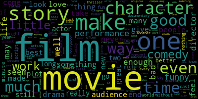
Let's build a word cloud of all the reviews first before we filter out for just top scorers in different categories and see what the most frequently mentioned words are. We define a function for plotting the word cloud to make it easy as possible to change out the source data.
def plot_wordcloud(series,output_filename='wordcloud'):

    from wordcloud import WordCloud

    wordcloud = WordCloud().generate(' '.join(series.astype(str)))

    wordcloud.to_file(output_filename + '.png')

    plt.imshow(wordcloud, interpolation='bilinear')

    plt.axis("off")

plot_wordcloud(text_data['clean_lemmatized'],'overall-wordcloud')
Next we create another function on top of the last, that'll slice the dataframe by the top N scorers and then plot the word clouds for us.
def plot_wordcloud_top_n(df,number_of_reviews,score_column,data_column,output_filename):
    sliced_df = df.nlargest(number_of_reviews,score_column)

    plot_wordcloud(sliced_df[data_column],output_filename)


plot_wordcloud_top_n(text_data,500,'0 Positive Sentiment Score','clean_lemmatized','positive-wordcloud')
plot_wordcloud_top_n(text_data,500,'0 Negative Sentiment Score','clean_lemmatized','negative-wordcloud')
plot_wordcloud_top_n(text_data,500,'0 Neutral Sentiment Score','clean_lemmatized','neutral-wordcloud')
Done! This is an extremely useful skill in natural language processing and powers a lot of recommendation engines you'll come across in real life.