Linear Regression: Under the Hood with the Normal Equation

Let's dive deeper into how linear regression works.

Linear regression follows a general formula:

Where \(\hat{y}\) is the predicted value, \(n\) is the number of features, \(x_i\) is the \(i^{th}\) feature value and \(\theta_n\) is the \(n^{th}\) model parameter. This function is then vectorised which speeds up processing on a CPU, however, I won't go into that further.

How does the linear regression model get 'trained'? Training a linear regression model means setting the parameters such that the model best fits the training data set. To be able to do this, we need to be able to measure how good (or bad) the model fits the data. Common ways of measuring this are:

• Root Mean Square Error (RMSE)
• Mean Absolute Error (MAE)
• R-Squared
• Adjusted R-Squared
• many others

From here on, we will refer to these as the cost function, and the objective is to minimise the cost function.

The Normal Equation

To find the value of \(\theta\) that minimises the cost function, there is a mathematical equation that gives the result directly, named the Normal Equation

Where \(\hat{\theta}\) is the value of \(\theta\) that minimises the cost function and \(y\) (once vectorised) is the vector of target values containing \(y^{(1)}\) to \(y^{(m)}\).

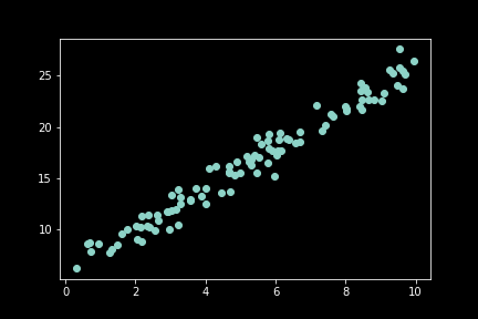
For example if this equation was run on data generated from this formula:

1
2
3
4

import numpy as np

X = 10 * np.random.rand(100,1)
y = 6 + 2 * X + np.random.rand(100,1)

Now to compute \(\hat{\theta}\) with the normal equation, we can use the inv() function from NumPy's Linear algebra module:

1
2

X_b = np.c_[np.ones((100,1)),X]
theta_best = np.linalg.inv(X_b.T.dot(X_b)).dot(X_b.T).dot(y)

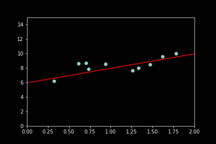
With the actual function being \(y = 6 + 2x_0 + noise\), and the equation found:

1
2

array([[ 5.96356419],
       [ 2.00027727]])

Since the noise makes it impossible to recover the exact parameters of the original function now we can use \(\hat{\theta}\) to make predictions:

1

y_predict = X_new_b.dot(theta_best)

With y_predict being:

1
2

[[ 5.96356419]
 [ 9.96411873]]

The equivalent code using Scikit-Learn would look like:

1
2
3
4
5

from sklearn.linear_model import LinearRegression
lin_reg = LinearRegression()
lin_reg.fit(X,y)
print(lin_reg.intercept_, lin_reg.coef_)
print(lin_reg.predict(X_new))

And it finds:

1
2
3

[ 5.96356419] [[ 2.00027727]]
[[ 5.96356419]
 [ 9.96411873]]

Using the normal equation to train your linear regression model is linear in regards to the number of instances you wish to train on, meaning you will need to be able to fit the data set in memory.

There are many other ways of to train a linear regression, some which are better suited for large number of features, these will be covered in later posts.