Logistic Regression with PyTorch
Posted on Sun 06 August 2023 in Python • 17 min read
In this post we'll go through a few things typical for any project using machine learning:
- Data exploration & analysis
- Build a model
- Train the model
- Evaluate the model
While this is a very high level overview of what we're about to do. This process is almost the same in any size & complex machine learning project.
We'll be using the iris dataset, which is a very famous hello world dataset in machine learning which contains 4 parameters which describe three species of flower (the iris flower). The sepal length & width, and the petal length & width are provided for 50 samples of each species. The sepals of a lower are the green leafy parts surrounding the flower head (which has the petals).
We'll also be trying to classify flowers into their species from their attributes using the logistic regression model. Logistic regression predicts the probability that something is either one thing or not based on the input variables.
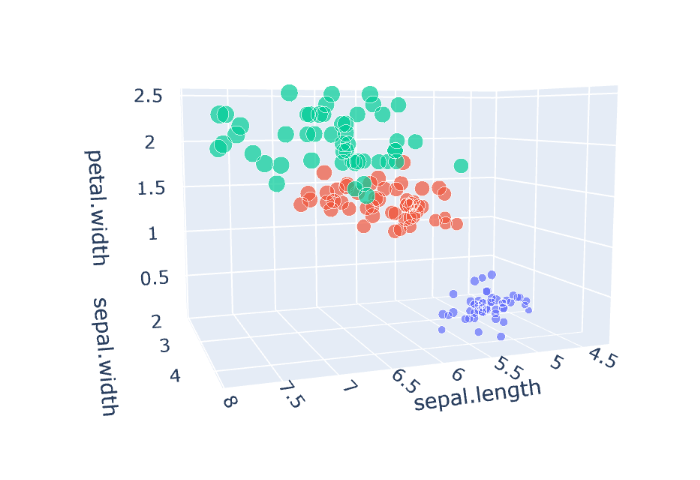
Let's take a look at our dataset visualised (below is how to produce this visual and an interactive version).
As always, we begin by importing the neccessary libraries/packages.
import pandas as pd
import plotly
import plotly.express as px
from IPython.core.display import HTML
import torch
import numpy as np
Data Exploration & Analysis
Time to dive in and take a lot at what we'll be working with. If this was a very rigourous project, we'd split the dataset into our train/validate/test set before even starting the validation as the modeller should never know what the test set looks like otherwise it introduces bias. Nevertheless in the pursuit of brevity we'll not do this here.
First off we'll take a peek at the first 5 rows of data so we can at least see what type of data they are (they are given as floats or numbers with decimal points) and the species is defined as a string. We can then check how many samples of each species we've been provided with the value_counts() method and finally we can take a look with describe to see common statistics about each attribute of our pretty little flowers.
iris = pd.read_csv('iris.csv')
print(iris.head())
print(iris['variety'].value_counts())
iris.describe()
Next we'll extract our species into a list for use later on.
species = list(iris["variety"].unique())

print(species)
Since the iris dataset has 4 input, and a single output feature, when we create a visualisation of all of this it'll be a 5 dimensional plot, and we'll use a scatter plot to represent this. By using the plotly package we can also make it interactive which is super handy for our 3D minds to visualise higher dimensional things.
fig = px.scatter_3d(iris[["sepal.length","sepal.width","petal.length","petal.width","variety"]],
                    x = 'sepal.length',
                    y = 'sepal.width',
                    z = 'petal.width',
                    size = 'petal.length',
                    color = 'variety',
                    opacity = 0.7)

fig.update_layout(margin = dict(l=0, r=0, b=0, t=0))

HTML(plotly.offline.plot(fig, filename='5d_iris_scatter.html',include_plotlyjs='cdn'))
To try and make it easier for our 3D minds, let's just plot all the dimensions in a single plot so we can see which features correlate with each other. To do this, we'll use a scatter matrix (also known as a pairwise plot).
fig = px.scatter_matrix(iris, dimensions=["sepal.width", "sepal.length", "petal.width", "petal.length"],color="variety")
HTML(plotly.offline.plot(fig, filename='5d_scatter_matrix.html',include_plotlyjs='cdn'))
By looking at this plots we can see that one species of flower is well separated from the others, while the others are mixed and overlapped for every pair of features. But if we use petal length and width that'll give us a nice separation between the species, and we'll train our first model on specifically these two features. This is known as feature selection.
Building the Model
Now it's time to prepare the data for our model, and create the model. We do this by creating tensors of the input and output data. A tensor is a general term for data with any amount of dimesion. A 2D tensor is commonly referred to as a vector, and a 1D tensor as a scalar, if that helps to think of these things as. Almost everything we'll come across in the world of machine learning makes use of tensors in one form or another.
selected_features = ['petal.length', 'petal.width']

input_columns_all = torch.from_numpy(iris[list(iris.select_dtypes('float').columns)].to_numpy()).type(torch.float32)
input_columns = torch.from_numpy(iris[selected_features].to_numpy()).type(torch.float32)
output_columns = torch.tensor(iris['variety'].astype('category').cat.codes)

print("Input columns all: ", input_columns_all.shape, input_columns_all.dtype)
print("Input columns: ", input_columns.shape, input_columns.dtype)
print("Output columns: ", output_columns.shape, output_columns.dtype)

data = torch.utils.data.TensorDataset(input_columns, output_columns)
As mentioned before, it's time to split up the dataset into a train, validation and test set. We'll use a split of 70-20-10 for these and make use of the random_split tool in PyTorch to randomize which records fall into each set.
Since we're using PyTorch we need to make this data iterable using DataLoader, and to enable many other features like shuffling, mapping and more. This also enables us to generate batches to train on.
split = 0.1
rows = iris.shape[0]
test_split = int(rows*split)
val_split = int(rows*split*2)
train_split = rows - val_split - test_split

train_set, val_set, test_set = torch.utils.data.random_split(data, [train_split, val_split, test_split])

train_loader = torch.utils.data.DataLoader(train_set, batch_size=16, shuffle = True)
val_loader = torch.utils.data.DataLoader(val_set)
test_loader = torch.utils.data.DataLoader(test_set)
Finally let's create the model! We do this by extending the Module class from within PyTorch, from the perspective of neural networks this could be seen as a single layer net. The class needs instructions on what to do when it's created and this is the __init__ dunder method. With a single 'layer' inside it which makes use of the Linear module from PyTorch. The Linear module will return probabilities for each dimension in the vector that we provide. This just means that if we give it 2 things to compare against, it'll give us the probability of either one. Next up we have the forward method, which returns the output of the model.
The next two methods, training_step and validation_step are what we'll be using for each respective step in the project process later on. training_step evaluates the given batch through the model and calculates the cross entropy loss for said batch. Cross entropy loss is the predicted probability compared to how far that is from the actual value.
validation_step repeats the same as training_step but also calculates the accuracy of the model by the count of correct predictions divided by the number of predictions.
class LogisticRegression(torch.nn.Module):
    def __init__(self, input_dimension, output_dimension):
        super(LogisticRegression, self).__init__()
        self.linear = torch.nn.Linear(input_dimension, output_dimension)

    def forward(self, x):
        outputs = self.linear(x)
        return outputs

    def training_step(self, batch):
        inputs, targets = batch
        outputs = self(inputs)
        loss = torch.nn.functional.cross_entropy(outputs, targets.long())
        return loss

    def validation_step(self, batch):
        inputs, targets = batch
        outputs = self(inputs)
        loss = torch.nn.functional.cross_entropy(outputs, targets.long())
        _, pred = torch.max(outputs, 1)
        # Calculate the number of correct predictions over the number of predictions
        accuracy = torch.tensor(torch.sum(pred==targets).item()/len(pred))
        # Detached is used here so the values aren't included in the gradient calculation
        return [loss.detach(), accuracy.detach()]
Now we need a way to:
- Evaluate how well our model is performing on a dataset
- Train the model on a dataset
def evaluate(model, loader):
    outputs = [model.validation_step(batch) for batch in loader]
    outputs = torch.tensor(outputs).T
    loss, accuracy = torch.mean(outputs, dim=1)
    return loss, accuracy
We fit the model by using the Adam optimizer (which could be replaced with something like gradient descent or otherwise), for a number of epochs (rounds) over the batches in the data. For each epoch, the losses from each batch are used to calculate the gradient, which in turn gets fed into the optimizer to tune the model parameters before moving onto the next batch. To ensure gradients aren't being messed up, we reset them before each batch and then we validate how well our model is performing on the validation set.
def fit(model, train_loader, val_loader, epochs, learning_rate, optimizer_function = torch.optim.Adam):
    history = {"loss" : [], "accuracy" : []}
    optimizer = optimizer_function(model.parameters(), learning_rate)
    for epoch in range(epochs):
        print("Epoch ", epoch)
        #Train
        for batch in train_loader:
            loss = model.training_step(batch)
            loss.backward()
            optimizer.step()
            optimizer.zero_grad()
        #Validate
        for batch in val_loader:
            loss, accuracy = evaluate(model, val_loader)
        print("loss: ", loss.item(), "accuracy: ", accuracy.item(), "\n")
        history["loss"].append(loss.item())
        history["accuracy"].append(accuracy.item())

    return history
At last we can train the model and see how well it performs on the test set!
epochs = 100
learning_rate = 0.01

model = LogisticRegression(len(selected_features), len(species))
fit(model, train_loader, val_loader, epochs, learning_rate)
loss , accuracy = evaluate(model, test_loader)
print("Evaluation result: Loss: ", loss.item(), " Accuracy: ", accuracy.item())
Evaluation result: Loss: 0.3645802438259125 Accuracy: 0.9333333373069763
As we can see after 100 epochs, we've got an accuracy of 93.3%! Now let's give it a go if it was using all the features (with no feature selection).
data_all = torch.utils.data.TensorDataset(input_columns_all, output_columns)

#train_split, val_split and test_split defined earlier
train_set_all, val_set_all, test_set_all = torch.utils.data.random_split(data_all, [train_split, val_split, test_split])

train_loader_all = torch.utils.data.DataLoader(train_set_all, 16, shuffle = True)
val_loader_all = torch.utils.data.DataLoader(val_set_all)
test_loader_all = torch.utils.data.DataLoader(test_set_all)

model_all = LogisticRegression(4, len(species))
history_all = fit(model_all, train_loader_all, val_loader_all, epochs, learning_rate)
loss , accuracy = evaluate(model_all, test_loader_all)
print("Evaluation result: Loss: ", loss.item(), " Accuracy: ", accuracy.item())
Evaluation result: Loss: 0.16669009625911713 Accuracy: 1.0
Wow! Using all the features got us 100% accuracy on the test set, this doesn't mean that always using all features will lead to this. It's a combination of balancing batch size, learning rates, epochs and more to get the right model for a situation.